Units
- in US units R value is ft^2 \circ F / BTU per hour
- in SI units R value is m^2 K / watt
Parallel
- If you have two conducting surfaces in parallel, the U-values add
- In parallel, the heat can take either path
Series
- If you have two conducting surfaces in series, the U-values add according to U_{total} = \left(\frac{1}{U_1} + \frac{1}{U_2}\right)^{-1}
- In series, the heat must take both paths
Bathtub model of heat flow
- What is the input?
- Now the drain is faster with greater temperature
Typical R and U values
- Window range (US R-values)
- R-1 for single pane
- R-12.5 for more advanced windows
- Wall range
- R-3.4 (2x4 no inssulation)
- R-12.7 (2x4 R-13 insulation)
- R-34.6 (2x6 R-21 insulation)
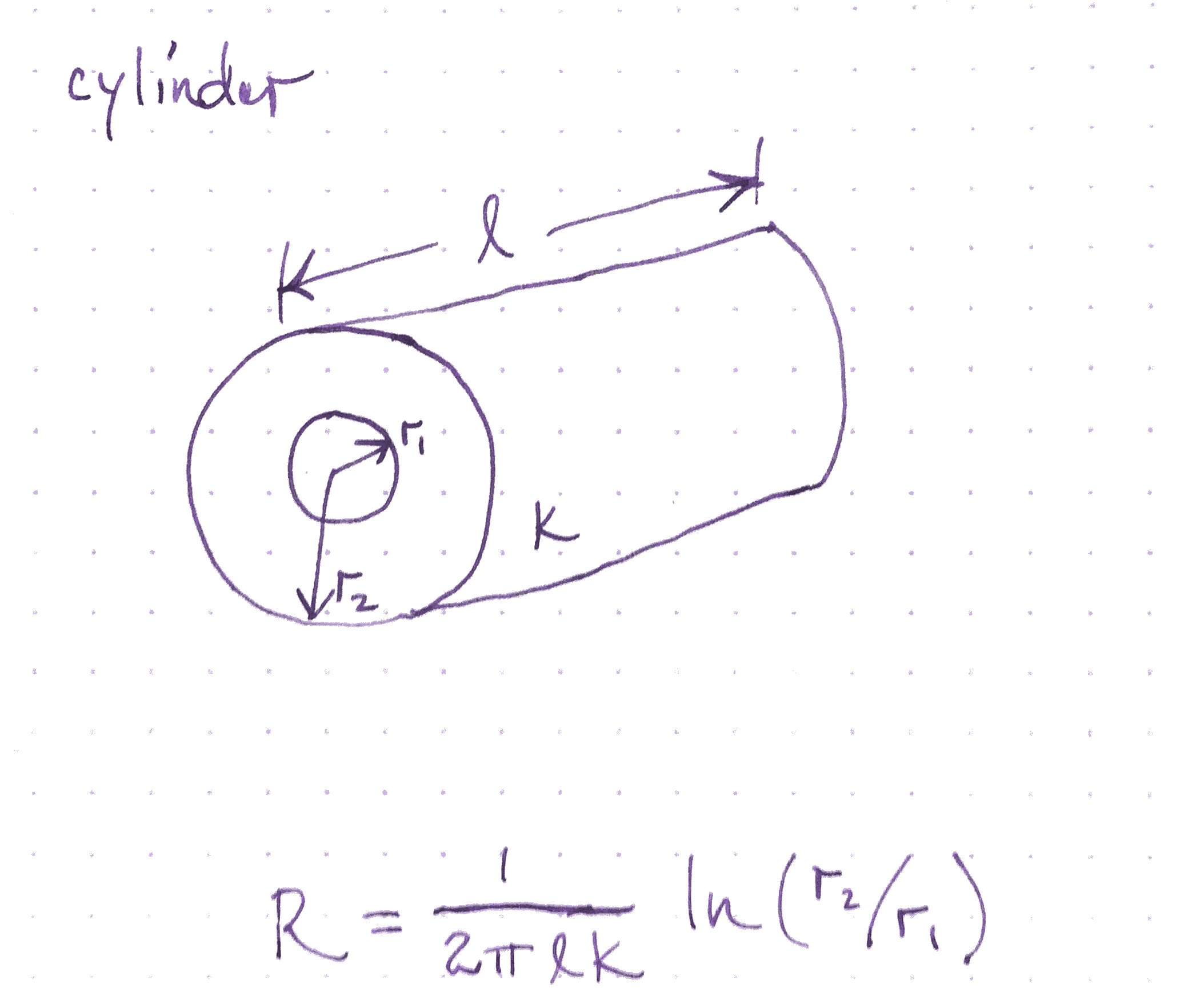
Cylindrical Insulator
Note that this R does not have the same dimensions as R-value. It has dimensions of temperature difference per unit power.
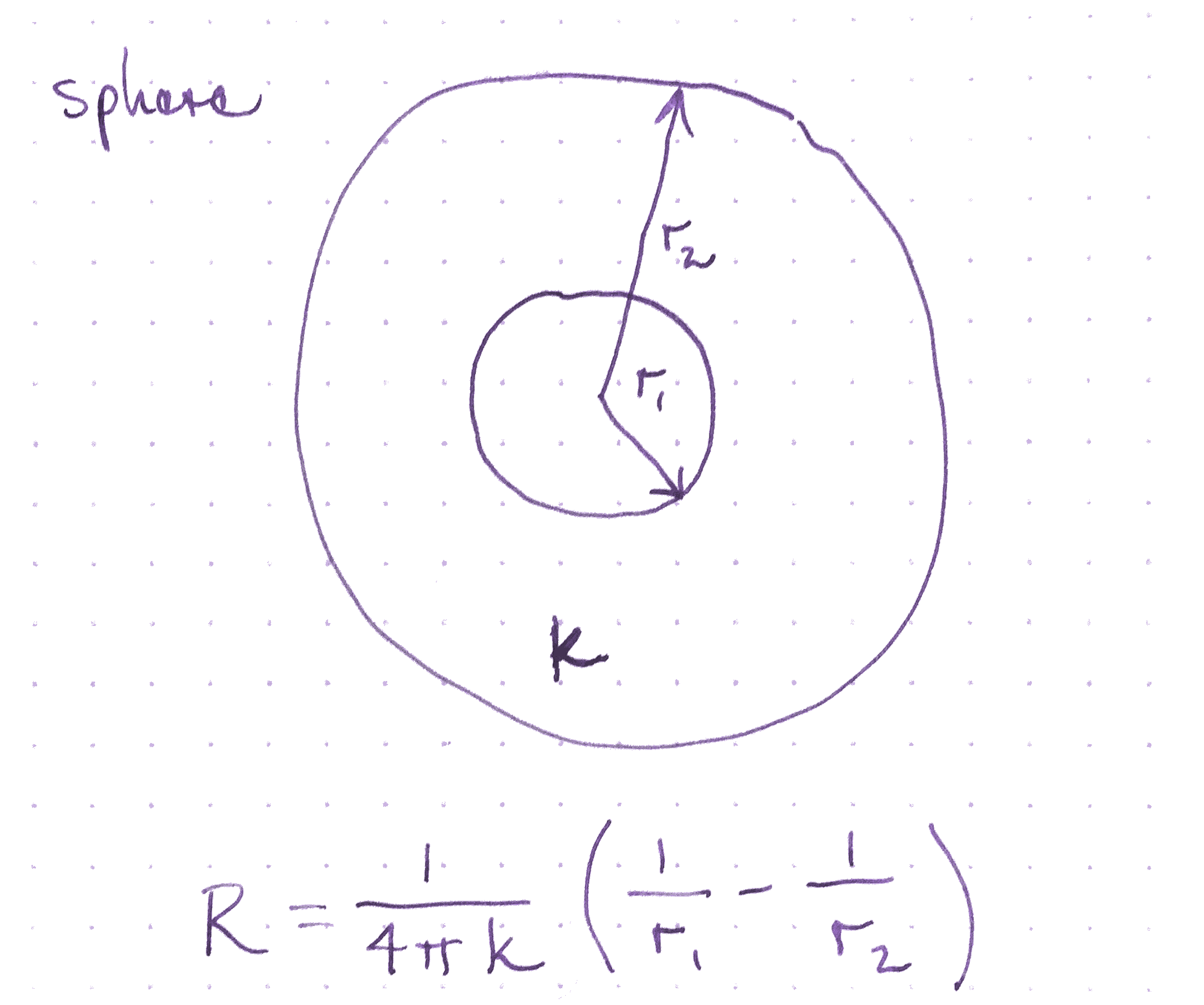
Spherical Insulator
Note that this R does not have the same dimensions as R-value. It has dimensions of temperature difference per unit power.
Typical UA values
- Residential Home ?
- Commercial Building ?
- Cooler ?
- Down Jacket ?
Activities
R-Value of SIP
Are the components of the SIP in parallel or series?
How do we find the properties of each?
Wood 0.15 watts per kelvin per meter
Polyurethane foam 0.02 watts per kelvin per meter
4.5 inch panel 13.8 R value
k_wood = 0.15 W/K/m
k_foam = 0.02 W/K/m
t_wood = 0.01 m
t_foam = 0.08 m

r_wood = t_wood/k_wood => 0.0667 m^2*K/W
r_foam = t_foam/k_foam => 4 m^2*K/W

r_SIP_SI = 2 * r_wood + r_foam => 4.1333 m^2*K/W

r_SIP_US = r_SIP_SI * 5.68 ft^2/m^2*F/K*W/BTU => 23.4773 ft^2*F/BTU
Convert R-values
Convert between a US R-value and a metric R-value.
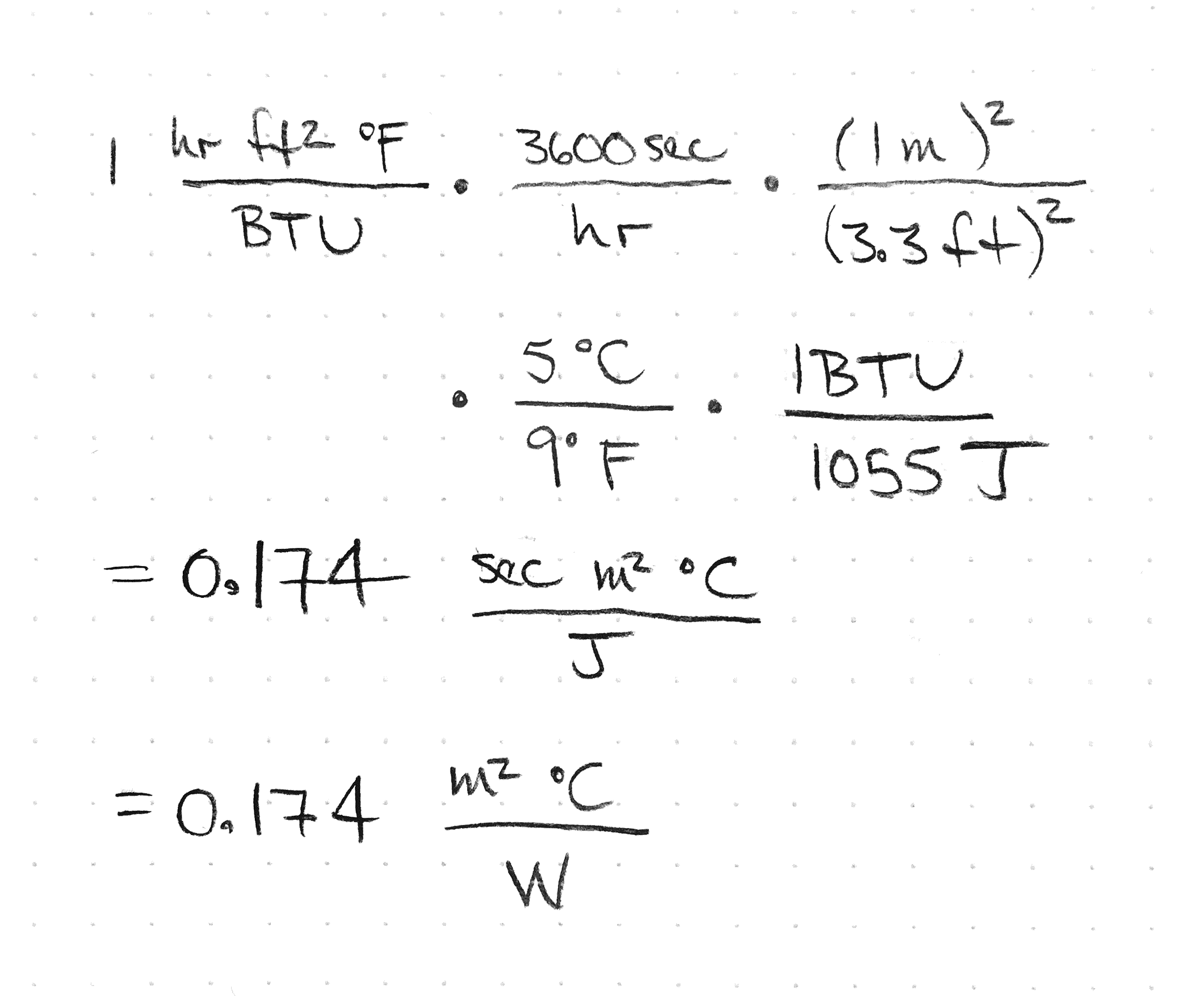
Once you learn how to do this, you can use the value you calculate as a conversion factor. This will help you convert more quickly.
Estimate Wall Loss in ETC
- What is the R-value?
- What is the total area of walls?
- How much power do we need to maintain the ETC one degree above the outside temperature?
Calculus Approach to Heat Loss through conduction
We calculate the temperature as a function of time of a heated object that loses heat to its surroundings through an insulation. We start with a lumped mass approximation with conductive heat loss through an insulator. Using the heat capacity of the object we have the relation
C = \frac{Q}{\Delta T}
Where C, the heat capacity is the product of the density, \rho, the volume of the object V, and the specific heat capacity of the material c.
C = \rho V c
Over a small time interval dt, the heat lost by the object as heat conducts away is the product of the temperature difference T - T_C, the thermal conductivity of the insulation, K and the time interval dt.
Q = K (T - T_C) dt
Substituting, we get
\rho V c = K (T - T_C) dt/dT
which we rearrange and integrate
\int_{0}^{t} \frac{K}{\rho V c} dt = \int_{T_0}^{T} \frac{dT}{T - T_C}
with initial conditions T = T_0 at t=0 and T=T at t=t. Integrating, we get
\frac{K}{\rho V c} t \bigg|_0^t = \ln(T - T_C) \bigg|_{T_0}^{T}
\frac{K}{\rho V c} t = \ln(\frac{T - T_C}{T_0 - T_C})
We exponentiate both sides and get
\exp(-\frac{K}{\rho V c} t) = \frac{T - T_C}{T_0 - T_C}
T = (T_0 - T_C) \exp (-\frac{K}{\rho V c} t) + T_C
The equation shows an exponential decay in temperature starting at T_0, the initial temperature of the object, decaying to T_C.
Discrete approach
We can also do this numerically with a discrete time period.
1-D form of Fourier’s Law
q_x = -kA\frac{\Delta T}{\Delta x}
- q_x dimensions of energy per time or power
- A dimensions of area
- k dimensions of power per distance per degree
- \Delta T is the temperature difference
- \Delta x is the thickness of the material