Heating and Cooling Degree Days

Concepts

Heating Degree Days
Cooling Degree Days
UA Product
Balance Point
Base Temperature
California Climate Zones
Typical Meteorological Year (Synthesized Data)
Historical Data

Heating and Cooling Degree Days

These metrics provide a simple way to distill a year’s worth of temperature data to a single number that is useful for energy estimations. We will see that the energy to heat and cool is proportional to the heating degree days (HDD) and cooling degree days (CDD) values.

UA Product

We recall that the UA product is the overall thermal conductance of the house telling us how much power must be applied to maintain a given temperature difference.

Balance Point

Any building has several internal sources of thermal energy. The lighting, occupants, and appliances all provide heat to the building. The balance point tells us what temperature difference the building will have between the outside temperature and the inside temperature without providing any energy from the heating system.

Base Temperature

This is the temperature we use to construct our temperature differences. It is related to the thermostat setting in the buildings. Some HDD calculation methods use the balance point, while others use a base temperature.

California Climate Zones

California designates 16 climate zones and compiles data for them to aid in climate-aware building design.

PG&E maintains a training document detailing these zones.

Historical Data

These are the actual recorded data from weather stations that have been compiled for analysis. These are often reported hourly.

Typical Meteorological Year (Synthesized Data)

Typical Meteorological Year (TMY) constructs a typical data set by taking the most typical month from the last several years and mixing them together in a data set. These data sets can be used by building designers to instead of historical data to design for a typical year.

Heating Degree Day Derivation

Block diagram of computational steps to create a heating or cooling degree day estimation. Source: Generated by author.

Recall that we can estimate the heat power for a structure’s envelope if we know the UA value and the temperature difference between the inside and the outside.

q = UA\Delta T

We assume for some interval of time \Delta t that the temperature is constant. Over that period of time, the energy moving from the inside of the envelope to the outside is

E = UA \Delta T \Delta t

Since outside temperatures change fairly slowly, we can estimate the energy by assuming the temperature is constant over the course of an hour. We call each temperature reading \Delta T_i and sum over our period of time (often a year).

E_{year} = \sum_{i=1}^{8760} UA \Delta T_i \Delta t

Since the UA value doesn’t change over time, we can write the UA outside of the sum. Note that we are only summing when the temperature difference is positive (or negative).

E_{year} = UA \sum_{i=1,\Delta T_{i}>0}^{8760} \Delta T_i \Delta t

The quantity in the sum is the degree days. Degree days are often tabulated using weather data and assumptions about the inside temperature of a building. We can also calculate degree day quantities if our assumptions are significantly different from the usual assumptions.

E_{year} = UA\ \textrm{HDD}

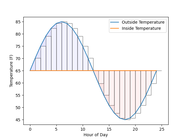
In the figure, we show a simple (unrealistic) temperature profile to demonstrate the areas representing degree-days and how our sum approximates them.

The blue shaded area represents cooling degree days where the outside temperature is higher than the desired indoor temperature. During this time, we would be cooling the structure. The red shaded area represents heating degree days where the outside temperature is lower than the desired indoor temperature. During this time, we would be heating the structure.

The rectangular outlines represent each of the hourly contributions to the sum. Our rectangles have a width of one hour and the height of the temperature difference at the beginning of the hour.

Approximation of the area under the curve using rectangles. Source: Generated by author.

Heating Degree Day Calculations

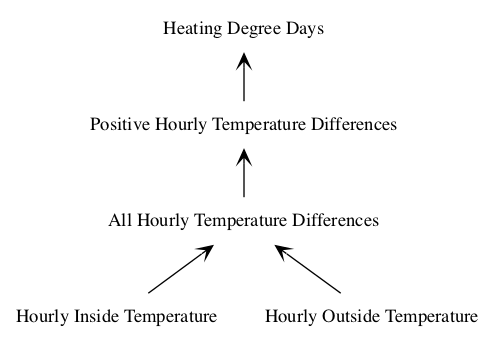
The basic steps of a calculation are

Obtain time series of outside temperature and base temperature
Create temperature differences
Discard negative temperature differences
Sum temperature differences

You must of course ensure that your calculations respect units and dimensions.

HDD and CDD methods

Integration method
- Uses high-resolution data to compute degree-days for each hour of day
Minimum–Maximum–Average approximations
- Uses low resolution data that may only have high and low daily temperatures

Degree Day Projections

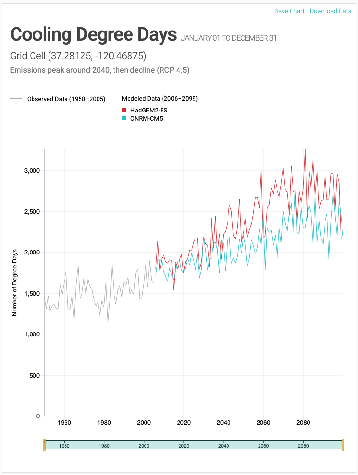
Climate scientists use physical and computer models to predict the earth’s climates assuming different amounts of carbon dioxide in the atmosphere. From these climate predictions, we can make predictions of the hourly temperatures for a given location. Then, from these hourly temperatures, we can make predictions of the degree days for a given area which tells us about the energy use for heating and cooling in those areas. Many areas predict increasing numbers of cooling degree days and decreasing numbers of heating degree days.

The Cal-Adapt website compiles predictions of cooling degree days and heating degree days over the next several decades using several climate models created by scientists.

You’ll notice that these predictions have variation from year to year but follow a trend. You can use visual or computational methods to estimate this slope and consider the implications of changing energy usage in the future.

Heating and Cooling Degree Days

Concepts