Conduction

Fourier’s Law

The fundamental formula for heat conduction in a material is Fourier’s Law.

q = -k \nabla T

• q has dimensions of power per unit area
• k has dimensions of power per distance per degree
• T is the temperature over space
• \nabla computes the direction and magnitude of the greatest temperature change

If you don’t speak vector calculus (most don’t) the formula tells you that

• the direction of heat energy flow is in the direction of decreasing temperature
• the amount of heat energy flow is proportional to a material property, k, and how abrupt the temperature change is.
• the minus sign tells us heat flows from hot to cold

Consequences

If a material is very hot on one side and cool on the other, there will be a large amount of heat flow.

If a material has a uniform temperature, there is no heat flowing.

Conduction

Fourier’s law covers many complex situations, but we can simplify this for our purposes.

Our simplification is called one-dimensional, steady-state conduction and it works for many real-life applications including buildings.

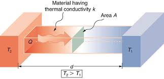
If we have

• a material (the bar in the middle)
• negligible heat loss on the edges of material
• a steady warm temperature on one side
• a steady cool temperature on one side
• and have waited until the temperature is no longer changing

We can use the following formula:

q = \frac{k A \Delta T}{L}

Where q is the heat power flowing across the material, k is the conductivity, A is the cross-section area of the material, and \Delta T is the temperature difference on the sides of the material, and L is the length of the material in the same direction as the heat flow.

What this means is that if I know the properties of a building wall and the inside and outside temperature, I can predict how much power is flowing across it.

Fourier’s Law, Buildings Form

Walls and buildings have several elements (walls, sheetrock, insulation, lumber, etc.). We can combine these into a single value called the UA value to perform power estimations for an entire building.

q = U A \Delta T

• q heat transfer dimensions of power
  • watts or BTU/hour
• U dimensions of power per area per degree temperature
  • watts/square meter/degree K
  • BTU/hour/square foot/degree F
• A dimension of area
  • square meters
  • square feet
• T dimension of temperature
  • Kelvin/Celsius
  • Fahrenheit

Quantity	Dimensions	Metric Units	Imperial Units
q heat transfer	power	watts	BTU / hour
U	power per area per temperature difference	watts / square meter / K	BTU / hour / square foot / F
R	area times temperature difference per power	square meter \cdot K / watt	square foot \cdot F \cdot hour / BTU
A	area	square meters	square feet
\Delta T	temperature difference	Kelvin or Celsius	Fahrenheit

R-value

U = \frac{1}{R}

R has

• dimensions of area times temperature difference divided by power
• square meters times celsius per watt
• square feet times fahrenheit times hour per BTU

Formula and Unit Rodeo

The equation above is presented in several forms with different units.

q = UA \Delta T

q = \frac{1}{R} A \Delta T

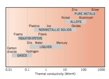
Conductivity

This graph shows the range of conductivities for different materials.

We can calculate the U-value of a material from

U = \frac{k}{L}

Examples

You have a wall with a UA value of 5 watts per Kelvin that is 25C on the surface of one side and 5C on the surface of the other side.

If the wall is at steady-state, how much heat is flowing in watts.

q = UA\Delta T q = 5 w/K \cdot (25C-5C) q = 100 W